이미지 임계처리
Goal
- 이미지 이진화의 방법인 Simple thresholding, Adaptive thresholding, Otsu’s thresholding에 대해서 알 수 있다.
cv2.threshold(),cv2.adaptiveThreshold()함수에 대해서 알 수 있다.
기본 임계처리
이진화 처리는 간단하지만, 쉽지 않은 문제를 가지고 있다. 이진화란 영상을 흑/백으로 분류하여 처리하는 것을 말합니다. 이때 기준이 되는 임계값을 어떻게 결정할 것인지가 중요한 문제가 됩니다. 임계값보다 크면 백, 작으면 흑이 됩니다. 기본 임계처리는 사용자가 고정된 임계값을 결정하고 그 결과를 보여주는 단순한 형태입니다.
이때 사용하는 함수가 cv2.threshold() 입니다.
-
cv2.threshold(src, thresh, maxval, type) → retval, dst¶ Parameters: - src – input image로 single-channel 이미지.(grayscale 이미지)
- thresh – 임계값
- maxval – 임계값을 넘었을 때 적용할 value
- type – thresholding type
- thresholding type은 아래와 같습니다.
- cv2.THRESH_BINARY
- cv2.THRESH_BINARY_INV
- cv2.THRESH_TRUNC
- cv2.THRESH_TOZERO
- cv2.THRESH_TOZERO_INV
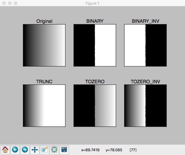
아래 예제는 각 type별 thresholding 결과입니다.
Sample Code
1 2 3 4 5 6 7 8 9 10 11 12 13 14 15 16 17 18 19 20 21 | import cv2
import numpy as np
from matplotlib import pyplot as plt
img = cv2.imread('gradient.jpg',0)
ret, thresh1 = cv2.threshold(img,127,255, cv2.THRESH_BINARY)
ret, thresh2 = cv2.threshold(img,127,255, cv2.THRESH_BINARY_INV)
ret, thresh3 = cv2.threshold(img,127,255, cv2.THRESH_TRUNC)
ret, thresh4 = cv2.threshold(img,127,255, cv2.THRESH_TOZERO)
ret, thresh5 = cv2.threshold(img,127,255, cv2.THRESH_TOZERO_INV)
titles =['Original','BINARY','BINARY_INV','TRUNC','TOZERO','TOZERO_INV']
images = [img,thresh1,thresh2,thresh3,thresh4,thresh5]
for i in xrange(6):
plt.subplot(2,3,i+1),plt.imshow(images[i],'gray')
plt.title(titles[i])
plt.xticks([]),plt.yticks([])
plt.show()
|
Note
여러 이미지를 하나의 화면에 보여줄때 plt.subplot() 함수를 사용합니다. 사용법은 위 소스나 Matplotlib Document를 참고하시기 바랍니다.
Result
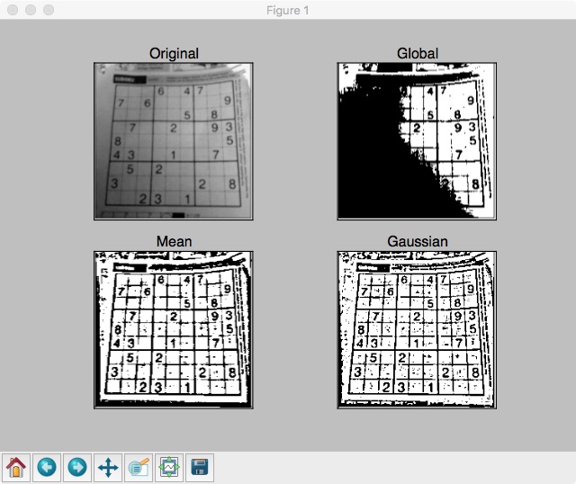
적응 임계처리
이전 Section에서의 결과를 보면 한가지 문제점이 있습니다. 임계값을 이미지 전체에 적용하여 처리하기 때문에 하나의 이미지에 음영이 다르면 일부 영역이 모두 흰색 또는 검정색으로 보여지게 됩니다.
이런 문제를 해결하기 위해서 이미지의 작은 영역별로 thresholding을 하는 것입니다. 이때 사용하는 함수가 cv2.adaptiveThreshold() 입니다.
-
cv2.adaptiveThreshold(src, maxValue, adaptiveMethod, thresholdType, blockSize, C)¶ Parameters: - src – grayscale image
- maxValue – 임계값
- adaptiveMethod – thresholding value를 결정하는 계산 방법
- thresholdType – threshold type
- blockSize – thresholding을 적용할 영역 사이즈
- C – 평균이나 가중평균에서 차감할 값
- Adaptive Method는 아래와 같습니다.
- cv2.ADAPTIVE_THRESH_MEAN_C : 주변영역의 평균값으로 결정
- cv2.ADAPTIVE_THRESH_GAUSSIAN_C :
Sample Code
1 2 3 4 5 6 7 8 9 10 11 12 13 14 15 16 17 18 19 20 21 22 23 24 25 26 | import cv2
import numpy as np
from matplotlib import pyplot as plt
img = cv2.imread('images/dave.png',0)
# img = cv2.medianBlur(img,5)
ret, th1 = cv2.threshold(img,127,255,cv2.THRESH_BINARY)
th2 = cv2.adaptiveThreshold(img,255,cv2.ADAPTIVE_THRESH_MEAN_C,\
cv2.THRESH_BINARY,15,2)
th3 = cv2.adaptiveThreshold(img,255,cv2.ADAPTIVE_THRESH_GAUSSIAN_C,\
cv2.THRESH_BINARY,15,2)
titles = ['Original','Global','Mean','Gaussian']
images = [img,th1,th2,th3]
for i in xrange(4):
plt.subplot(2,2,i+1),plt.imshow(images[i],'gray')
plt.title(titles[i])
plt.xticks([]),plt.yticks([])
plt.show()
|
Result
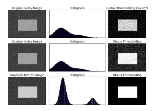
Otsu의 이진화
지금까지 thresholding처리를 하면서 임계값을 사용자가 결정하여 parameter로 전달하였습니다. 그렇다면 그 임계값을 어떻게 정의해야 할까요? 가장 일반적인 방법은 trial and error방식으로 결정했습니다. 그러나 bimodal image (히스토그램으로 분석하면 2개의 peak가 있는 이미지)의 경우는 히스토그램에서 임계값을 어느정도 정확히 계산 할 수 있습니다. Otsu의 이진화(Otsu’s Binarization)란 bimodal image에서 임계값을 자동으로 계산해주는 것을 말합니다.
적용 방법은 cv2.threshold() 함수의 flag에 추가로 cv2.THRESH_STSU 를 적용하면 됩니다. 이때 임계값은 0으로 전달하면 됩니다.
아래 예제는 global threshold값, Otsu thresholding적용, Gaussian blur를 통해 nosise를 제거한 후 Otsu thresholding적용 결과 입니다.
Sample Code
1 2 3 4 5 6 7 8 9 10 11 12 13 14 15 16 17 18 19 20 21 22 23 24 25 26 27 28 29 | import cv2
import numpy as np
from matplotlib import pyplot as plt
img = cv2.imread('images/noise.png',0)
# global thresholding
ret1, th1 = cv2.threshold(img, 127, 255, cv2.THRESH_BINARY)
ret2, th2 = cv2.threshold(img, 0, 255, cv2.THRESH_BINARY+cv2.THRESH_OTSU)
blur = cv2.GaussianBlur(img,(5,5),0)
ret3, th3 = cv2.threshold(img, 0, 255, cv2.THRESH_BINARY+cv2.THRESH_OTSU)
# plot all the images and their histograms
images = [img, 0, th1, img, 0, th2, blur, 0, th3]
titles = ['Original Noisy Image','Histogram','Global Thresholding (v=127)', 'Original Noisy Image','Histogram',"Otsu's Thresholding", 'Gaussian filtered Image','Histogram',"Otsu's Thresholding"]
for i in xrange(3):
plt.subplot(3,3,i*3+1),plt.imshow(images[i*3],'gray')
plt.title(titles[i*3]), plt.xticks([]), plt.yticks([])
plt.subplot(3,3,i*3+2),plt.hist(images[i*3].ravel(),256)
plt.title(titles[i*3+1]), plt.xticks([]), plt.yticks([])
plt.subplot(3,3,i*3+3),plt.imshow(images[i*3+2],'gray')
plt.title(titles[i*3+2]), plt.xticks([]), plt.yticks([])
plt.show()
|
Result